The Incumbency Advantage and Time For Change Model
Oct 2, 2020
It is common knowledge in the political science space that incumbents tend to perform better than non-incumbents in elections. In fact, since 1932, only three presidents have failed their re-election bids. But such begs the question, how does this incumbency advantage affect election predictions? In this blog, I will explore this question, first by analyzing the historical popular vote share of incumbent candidates vs. non-incumbents. Then, I will highlight how the incumbency advantage is factored into models like the “time-for-change” model. Finally, I will compare the time-for-change model to a model from my previous blog and evaluate such on their in-sample fit and out-of-sample error.
The Relationship between a Candidate’s Incumbency Status and Two-Party Popular Vote Share
| Incumbency Status vs. Two-Party Popular Vote Share (1948-2016) |
|---|
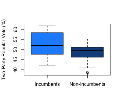 |
To understand how incumbency status can affect election predictions, it is necessary first to understand the relationship between a candidate’s incumbency status and two-party popular vote share. The boxplots above display historical trends for such, stratifying candidates based on their incumbency status and displaying each set of candidates’ two-party popular vote shares from 1948 to 2016. Some of the major takeaways include:
-
Higher vote share for incumbents. The boxplots indicate that an incumbent candidate’s two-party popular vote share has historically been higher than a non-incumbent candidate’s vote share. This is evident given the greater median vote share for incumbent candidates relative to non-incumbent candidates, which fits in with the commonly held notion that incumbents perform better than non-incumbents.
-
Greater spread for incumbets. The graphic also illustrates a greater spread of two-party popular vote share figures for incumbent candidates than non-incumbent candidates. In other words, while the middle 50% of popular vote shares fall between 48.24% and 58.10% for incumbent candidates, the middle 50% of popular vote shares for non-incumbent candidates only falls between 46.21% and 51.14%.
The Time-For-Change Model
The time-for-change model is a linear regression model that leverages the afromentioned incumbent advantage among other variables to predict an incumbent party candidate’s two-party popular vote share (PollyVote)
The first component of this model is the election-year second-quarter GDP. In my second blog, I established how this fundamental variable is the most predictive economic measure relative to all others; thus, its inclusion in the time-for-change models is justified.
The second component is the incumbent president’s net approval rating in the latest Gallup poll. This holds the incumbent party candidate’s popular vote share relative to the current serving president’s job approval ratings, given voters view elections as a referendum on parties currently holding power.
The third component is the incumbency status. As previously mentioned, this allows the model to factor in the incumbency advantage in election predictions. More specifically, the model factors that incumbency status is associated with a 2.87% increase in the incumbent party candidate’s two-party popular vote share.
Ultimately, the time-for-change model has been historically successful, with such model only having a true out-of-sample popular vote prediction error of 1.7% since 1992. Nevertheless, it’s necessary to evaluate such model against others to determine its predictive ability.
Evaluating Prediction Models
| Model | Variable(s) | R-squared | Mean Squared Error | Leave One Out Validation | Cross Validation |
|---|---|---|---|---|---|
| Time-For-Change | Second Quarter GDP, Net Approval, Incumbency Status | 0.68 | 2.87 | -2.86 | 1.45 |
| Week 3 | Average Support | 0.72 | 2.50 | -0.91 | 1.56 |
As the table demonstrates, I will compare the time-for-change model to my previous best model (Week 3), a linear regression model based on average support. I will evaluate each model’s predictive ability of an incumbent party candidate’s two-party popular vote share based on their in-sample fit and out-of-sample error, with the variables in the table giving insight into each of these metrics.
In-sample fit. Given the relatively high r-squared and low mean squared error values, the model with the best in-sample fit is the week 3 model.
Out-of-sample error. Although my week 3 model has a lower leave-one-out validation value, the model with the least out-of-sample error is the time-for-change model. This is due to such model having a lower cross-validation value than my week 3 model, which is more indicative of out-of-sample error given it averages multiple leave-one-out validations.
Overall, both models have fair in-sample fit and out-of-sample error. However, given the time-for-change model has a lower out-of-sample error, I would ultimately consider the time-for-change model more predictive of an incumbent party candidate’s two-party popular vote share than the week 3 model.
Predictions for 2020
The time-for-change model’s prediction for the incumbent party candidate’s (Trump) two-party popular vote share is 31.76%. This is substantially lower than the prediction associated with my week 3 model, which stands at 50.04%. One possible reason for this discrepancy is the time-for-change model’s inclusion of second-quarter GDP, which is drastically lower in 2020 than in any previous election year post-1948.
The prediction interval associated with each model’s predictions also differed, with the time-for-change model’s prediction interval, ranging from 12.15% to 51.36%, being substantially wider than my week 3 model’s interval, which ranged from 43.8% to 56.28%.
Ultimately, the differences in the predictions associated with both models underscore the uncertainty in predicting the 2020 incumbent party candidate’s vote share. Such predictions also indicate the smaller role incumbency might play in the 2020 election, given its small effect on the time-for-change model’s low two-party vote share prediction for Trump.
Final Takeaways
Overall, my analysis has demonstrated while there is an incumbency advantage in presidential elections, given incumbents have historically performed better than non-incumbents, such will not play a significant role in the 2020 election, given the time-for-change model’s low prediction for Trump. Moreover, while a comparison between the time-for-change model and my week 3 model demonstrates that the time-for-change model has the greater predictive ability, its inclusion of second-quarter election year GDP drags its overall prediction for 2020 down. Future models should consider leveraging these factors in the construction of new predictive models for 2020.